Introduction

In machine learning, working in high-dimensional spaces is often either computationally intractable or does not yield good practical results. Firstly, the curse of dimensionality (which helds that the more features/dimensions a data sample has, the more samples we need in order to accurately model the distribution of the data) compels us to find more data, thus making training and inference prohibitively expensive. Secondly, it is often the case that information in real-world data is embedded in only a few dimensions. Having more dimensions raises modeling issues by complicating the problem and leading to a lack of generalization. Thus, one may often want to perform dimensionality reduction before modeling, in order to capture the most essential features of the input data. Enter PCA.

PCA - intuition

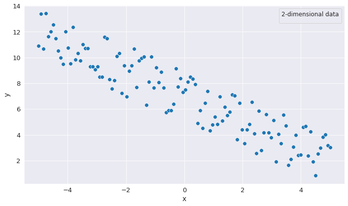
PCA is an algorithm that tries to identify the most import dimensions of the input data (principal components) and remove the unnecessary ones. But how does PCA identify the unnecessary dimensions? For that, let us have a look at the following image.

An example of two-dimensional data that is negatively correlated (whenever x increases, y decreases) in its raw form.

Were we to look at the data from the perspective of the 2 coordinates individually, we would be tempted to assume that each corresponding dimension contains a substantial amount of data and is indispensable. However, were we to choose a different system of coordinates, we could see a disproportion insofar as the quantity of information might not as dispersed as we would think it is.

The same data as above, but represented using a different system of coordinates.

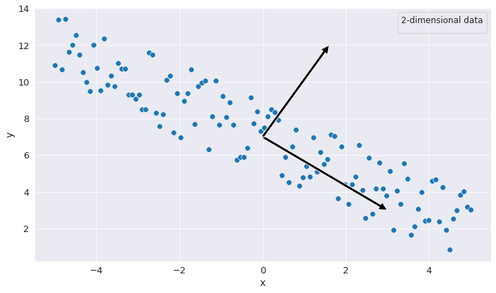
If we look at the figure from above, we see that, across one of the axes the information is not as widely spread as in the first system of coordinates. What this means in practice is that we may want to get rid of this dimension for the sake of preserving the most relevant information for modeling and so perform some dimensionality reduction on the input data. Seemingly we have achieved our goal of reducing the dimensionality of the data, even though the data was initially not obviusly reducible. The question, however, of finding the appropiate system of coordinates in which one could perform dimensionality reduction remains open.

PCA - In Detail

Let us delve into the more intricate details of PCA in order to see how one could find the appropiate system of coordinates.

Reducing the Covariance of the Data

The tenet of finding such a system of coordinates is the covariance between the dimension of the input data. In the last image from above, we see that the input dimensions have a correlation of 0. Therefore, we can examine the spread of each of the dimensions individually and decide which ones do not contain critical information for modeling and thus can be removed. Ideally, we want to find such a decorrelated system of coordinates for any input data that we have. Fortunately, there is a theoretically sound way of finding it. But, to begin with, let us first look at the covariance of the input data.

Let us assume, for the sake of generality, that we have a d-dimensional input data.

The covariance matrix of \(X\) would be a \(D x D\) matrix of the form:

As an observartion, this is a square and symmetric matrix. We know that real symmetric matrices are diagonizable and always admit a spectral decomposition. Hence, decomposing our matrix \(\Sigma_{X}\) leads to:

In the decomposition, \(\Lambda\) is a diagonal matrix, that has 0 as values for all elements besides the ones that reside on the diagonal. But this is exactly what we wished for before! A covariance matrix, where all the covariances between every two distinct dimensions are 0. Now, the question that remains is how do we transform our data such that it has this covariance?

Transforming the Input

We know that eigendecomposition finds a new vector space (where the eigenvectors form an orthonormal basis). One way would be to project the vectors in our original data matrix onto the newly found vector space. For that, multiplying with \(\Gamma\) should suffice. Therefore, our new data would be:

The new data would have the covariance as found above: \(\Lambda\). To make sure, let us redo the calculation. For simplification and without loss of generalization, let us consider a \(2 x 2\) input matrix:

This can be rewritten as:

After transformation:

Then, the covariance matrix of the transformed input would be:

We would expect at this point that \(Cov(Y_1, Y_2) = 0\) and \(Cov(Y_2, Y_1) = 0\). For the sake of keeping things short enough, we will only see that \(Cov(Y_1, Y_2) = 0\). The demonstration is similar for \(Cov(Y_2, Y_1)\).

We know that the dot product is associative with respect to a scalar: \(c(a \cdot b) = a \cdot (cb)\). We can use this in our case as well, since \(X^1w_1\) is a scalar and thus \(X^1w_1(X^1w_2) = X^1(X^1w_1w_2)\). But \(w_1w_2 = 0\), due to the orthonormality property of the eigenvectors. Thus, the whole thing is \(0\). More specificially:

Both terms are 0 for the reason mentioned above and thus:

Similarly one can show that \(Cov(Y_2, Y_1) = 0\) and thus the covariance between every two dimensions of the projected input is 0.

Reducing the Input Dimensionality

So far, we have shown that we can find a new system of coordinates (algebraically, we can perform a change of basis) such that the covariance between every two dimensions is 0. Now, what we ought to do is to choose which dimensions we are going to keep and which we are going to drop. As a rule of thumb, one could look at the variance across each dimension in the \(\Lambda\) matrix (which corresponds to an eigenvalue) and decide which dimensions have a small variance. If the variance is reasonably small (up to be decided by the person who does the modelling) then we can give up on that dimension. This has repercussions on the space on which we project the input though. If we project on a lower-dimensional space, then one has to drop an eigenvalue and an eigenvector. Therefore, instead of multiplying by \(\Gamma\), one has to reduce the columns from \(\Gamma\) that correspond to the smallest eigenvalues, obtain a new \(\Gamma_{trunc}\) and perform the projection in the same way, by doing \(X \cdot \Gamma_{trunc}\).

In this way, one can perform dimensionality reduction by reducing the least informative dimensions.