Introduction

In machine learning, it is often the case that one ends up (after various modeling steps) with an optimization problem. For instance, in SVMs, one has to find the optimal hyperplane that maximizes the margin. Furthermore, optimization is generally potentially complicated due to constrains that one imposes on the optimal point that is to be found. According to the taxonomy of optimization problems, this type of problems is part of the class of constrained optimization problems. If the objective function that one wants to optimize (and typically minimize) is convex, there are two major techniques that are typically used in order to achieve this.

The Lagrange multipliers

Let us assume we have a convex objective function \(f(x)\) that we want to optimize (in particular, we will talk about minimization, since any maximization problem can be reduced to a minimization problem). Furthermore, there are a couple of additional constraints that we may want to impose on the minimum that we find. For now we will just focus on affine and equality constraints, since the method that we are going to investigate offers guarantees only for this class of constraints. To sum up, the problem that we’re looking at is of the form:

, where \(f(x)\) - convex and \(g_i(x)\) - affine constraints.

Intuition

Let us assume we want to optimize \(f(x)\) without any constraints. To do this, one naturally looks at the gradient. We can just enforce \(\nabla f(x) = 0\) and we find the \(x\) at which this holds (assuming the function is convex). With the constraints, however, this idea does not work anymore, since the minimum of \(f(x)\) may not fulfil \(g_i(x) = 0\) for some \(i\). Geometrically, in order to visualize this, let us assume (without loss of generality) we have only one constraint.

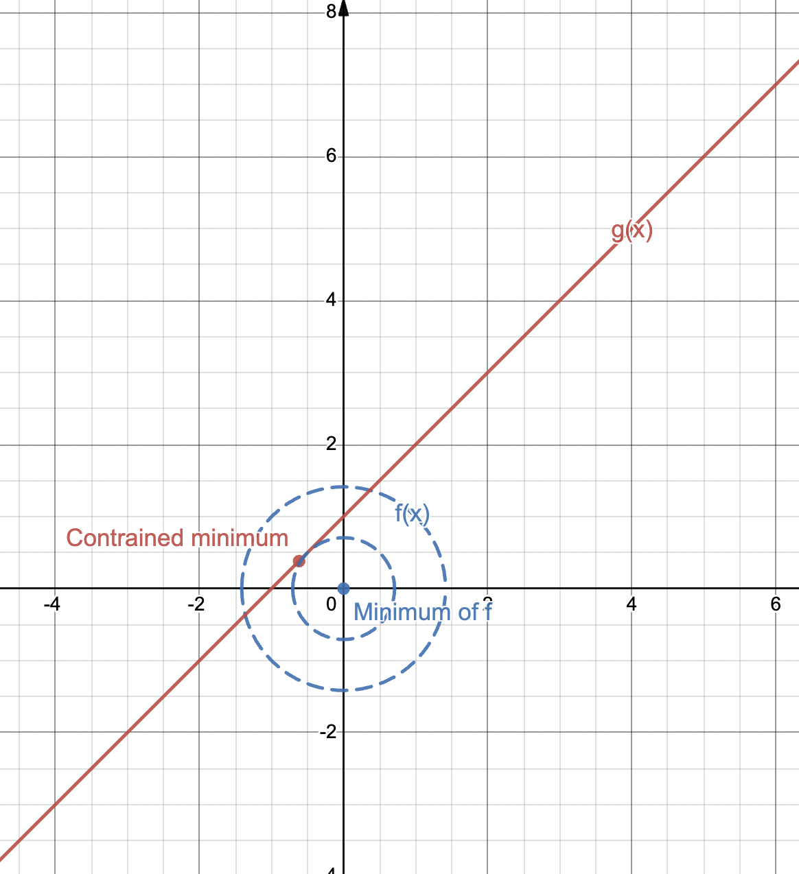
An example where the minimum of an objective function is not identical to the constrained minimum (for simplification, the contour plot of a higher dimensional function onto a 2D space is shown). Made with © Desmos.

As we can see in the picture from above, the constrained minimum does not coincide with the minimum of \(f\) and it is actually materialized at a point towards the upper-left side of the minimum of \(f\). And, more importantly, \(\nabla f(x_{min})\) is not \(0\). To find this type of points analytically, Lagrange figured out that, instead of looking at where the gradient is 0, one should look instead at where the gradients of the constraint function and the objective function are parallel. This intuition is very revealing, due to the fact that the set of points among which we’re searching our minimum must be the set of points on the constraint line. If we take a certain point on a line and there exists another point that leads to a better minimum on the same line, then the gradient of \(f\) must point towards it. Therefore, it cannot be perpendicular on the tangent line to the curve at this point. Meanwhile, the gradient of the constraint function is always perpendicular on the line (one can also visualize it as the normal vector of the line). Similarly, if there is no other point better than the current point, then the gradient of \(f\) must be perpendicular on the tangent (there is no better minimum on the constraint line, but there is one potentially outside of it - however, we are not interested in it). But since this point is on the constraint line, the gradient of \(g\) (the constraint function) must also be perpendicular on the constraint line (and on the tangent, by extension). Therefore, by ensuring that the two gradients are parallel, we are sure that there cannot be a more optimal point than this. This can be visualized as follows:

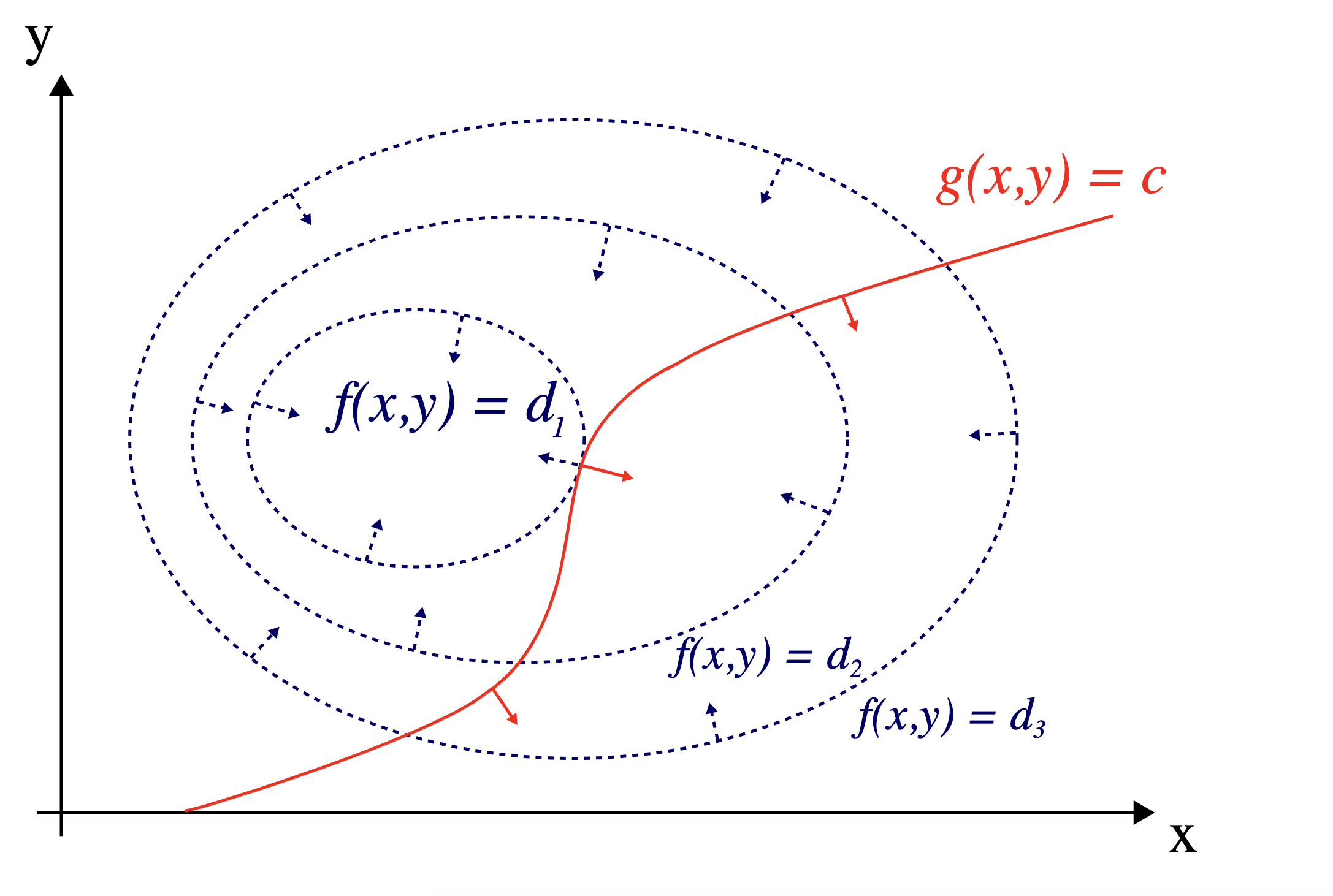
An example of Lagrange multipliers for 2D objective and constraints functions (© https://en.wikipedia.org/wiki/Lagrange_multiplier).

Formalism

Analytically, this parallelism can also be described with the following equation:

\(\lambda\) is a scalar that ensure that the vector gradients have the same direction, but not necessarily the same length. The second equation ensures that the point is on the constraint line. By solving this equation, one can find both the optimal \(x\) and \(\lambda\). This can also be naturally extended to multiple constraints \(g_i(x)\), \(\forall i \in {1..N}\).

The Lagrangian

Problems in practice can be even more complex than what we’ve seen before. A natural extension of the method above that makes use of the Lagrangian will be introduced and justified.

Justification

In practice one typically encounters optimization problems, for which the constraint functions can be inequalities. For these situations, an extension of the method would be required. To understand why, let us have a look at the example from above again. Assume we have the objective function \(f(x)=\frac{x^2}{2}+\frac{y^2}{2}\) with one constraint \(2 \cdot x - y \leq 1\) (without loss of generalization we consider only constraints of this type; constraints of the type \(c(x) \geq a\) can be reformulated into \(c'(x) \leq -a\), where \(c'(x)=-c(x)\)), which can be rephrased as follows:

In the equations from above, I have rewritten the constraint as \(g(x) = 2 \cdot x - y - 1\). Let us have a look at the graph of these functions.

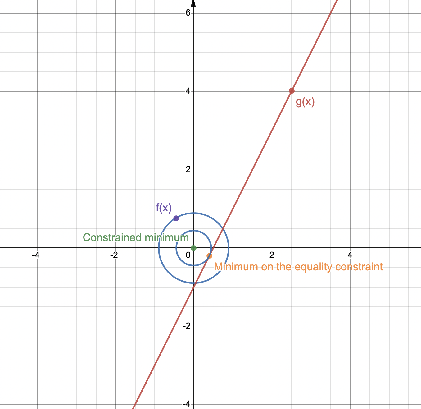
An example of optimization problem where the optimal solution is different for inequality constraints, compared to equality constraints. Made with © Desmos.

If one looks at the chart from above, one sees that the minimum of the problem with an inequality constraint does not coincide with the minimum for the problem with an equality constraint. By imposing \(g(x) = 0\), the method of Lagrange multipliers would find the minimum on the constraint line. However, that does not coincide with the real optimum, which is actually the same as the minimum of \(f(x)\). For this reason, an adaptation of the method of Lagrange multipliers is required in order to make it work for inequality constraints.

Intuition

One can also see the finding of an optimum under inequality constraints from a different angle. One could engineer a surrogate function that penalizes the points for which the inequality constraints do not hold. This can be mathematically translated as follows:

This function that we just defined is called the Lagrangian. It is essentially a reformulation of the method of Lagrange multipliers for equality constraints that I described above. Its mechanics can be best understood when we look at it for \(\lambda \gt 0\). \(g(x)\) is always positive for points that do not fulfill the constraint. Hence, \(\lambda \cdot g(x)\) will add a penalty to points outside of the constraint. Conversely, \(\lambda \cdot g(x)\) will be negative for points that fulfil the constraint, since \(g(x) \lt 0\). This leads to lowering the value of \(L(x, \lambda)\) for points that overfulfil the constraint (\(g(x) \lt \lt 0\)).

Now, to solve this problem, one has to find a \(\lambda\), which is big enough to penalize all the points that do not fulfill the constraint, but which also does not overly reward points that “overfit” on the constraint, i.e. points for which \(g(x) \lt \lt 0\).

Formalism

Analytically, this can be phrased as finding \(\min_{x} f(x) + \lambda g(x)\) for every possible \(\lambda\) (which can be formulated as \(g(\lambda) = \min_{x} f(x) + \lambda g(x)\)) and then optimizing over \(\lambda\), by finding \(\max_{\lambda} g(\lambda)\). Optimizing \(g\) is called, in literature, the dual problem. So, in a nutshell, finding the minimum under the constraints can be rephrased as:

This also means finding the saddle point of the Lagrangian. To see why this works, let us look at an example. To keep things simple, we will look at an optimization problem with one inequality constraint and one variable functions only (without loss of generality):

The chart of this function would be:

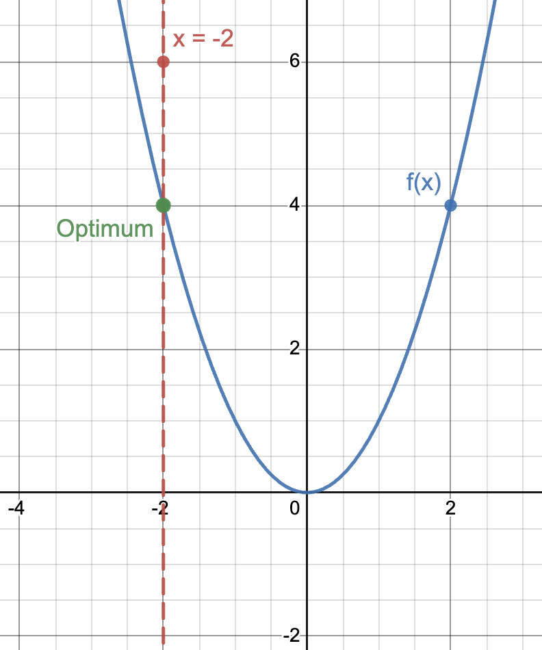
An example of optimization problem where we have a convex objective and one inequality constraint. The constrained area is to the left of the line $$x = -2$$. Made with © Desmos.

The optimum that we’re interested in is at \(x = -2\). Now, let us look at the dual function for certain values of \(\lambda\).

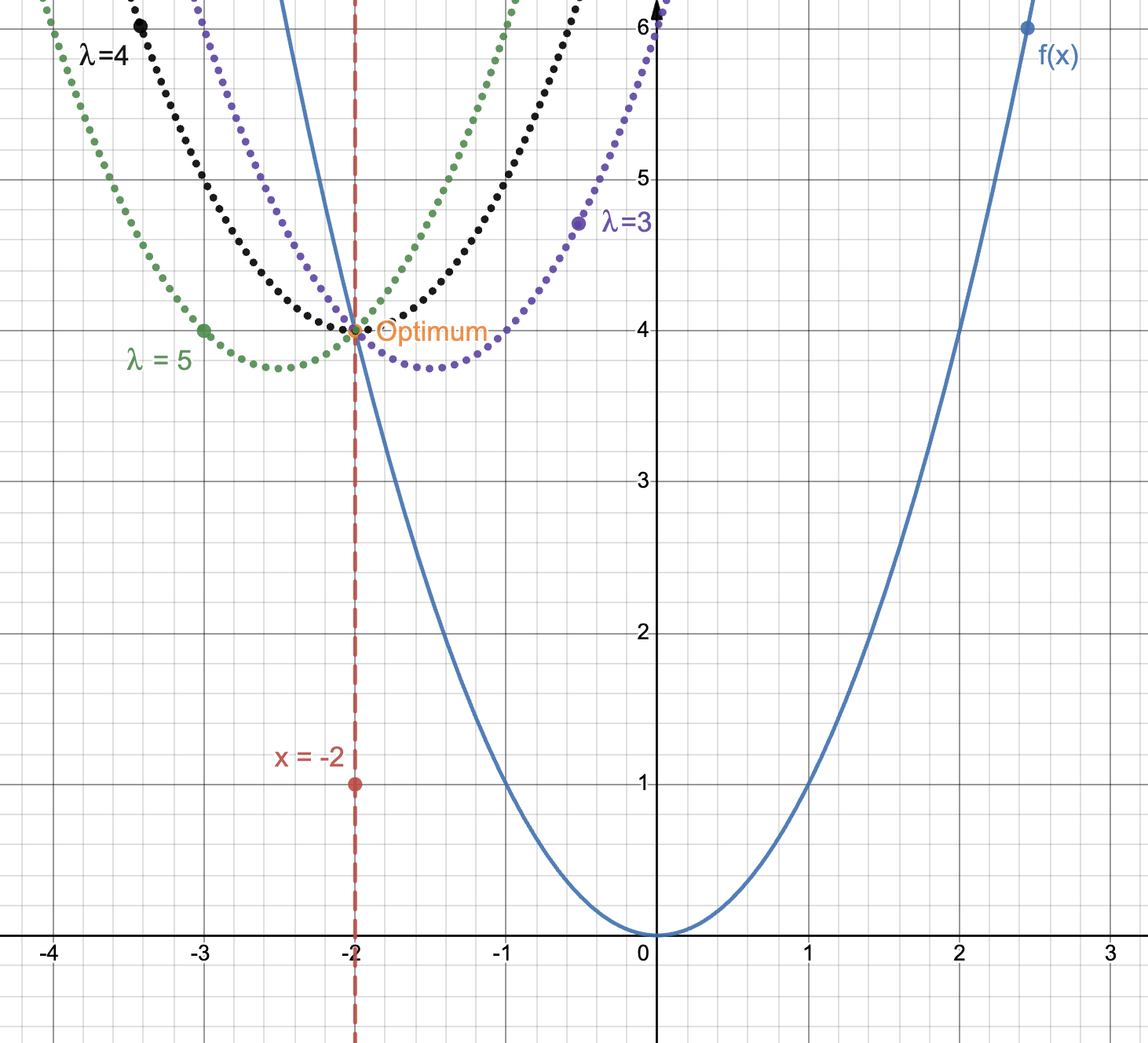
The same problem from before, where we see the dual for multiple values of lambda. Made with © Desmos.

As one can see, the more we increase \(\lambda\), the more the unconstrained minimum of \(f\) (at \(x=0\)) is penalized. That is the reason why the constrained minimum (\(g(\lambda)\)) has to move to the left of the unconstrained minimum, so that it is closer to the constraint line. At the same time, the more we move to the left (up to a certain point as we will see), the larger the value of the constrained minimum (than the previous constrained minimum) is. This is due to the fact that we are in a regime where the first terms of \(g\) is dominant (\(f(x)\)) and moving even slightly to the left entails moving farther from the unconstrained minimum of \(f\) and thus having higher values for \(f(x)\).

However, by going farther and farther to the left and entering the area where the constraint is fulfilled (see \(\lambda=5\) in the figure from above), we enter a regime where the second term of \(g\) is dominant (\(\lambda g(x)\)). This term is negative, since the constraint is fulfilled. By increasing \(\lambda\), we only increase the influence of this term and thus generating smaller and smaller constrained minima (up to \(-\inf\)), that are far from what we are interested in.

The point we are actually interested in is at the intersection of the 2 regimes. \(\lambda\) should be high enough such that all points to the right of the constraint line are sufficiently penalized and can not be optima anymore (the first term of \(g\) is not overly influential), but small enough such that the points that are well into the constrained area are not overly appreciated (the second term of \(g\) is not overly powerful). This point in which we are interested corresponds to \(\lambda=4\) in the figure from above. It also corresponds to the point for which \(g(x)=0\) (exactly on the edge of the constrained area). Finding this point corresponds to finding the maximum of \(g\) and finding the maximum of \(g\) entails solving \(\max_{\lambda}\min_{x} L(x, \lambda)\), thus the saddle point of the Lagrangian.

This method, like the one of the Lagrange multipliers for equality constraints, can naturally be generalized to multiple constraints.

Guarantees

Unfortunatelly, this algorithm does not necessarily provide theoretical guarantees for all class of problems. For instance, if the problem is not convex, then solving the dual will find a point that will be at a certain gap than the real optimum. The KKT conditions provide theoretical gurantees for the optima that are found, by defining (what is called in literature) strong duality (no gap between the optimum that is found and the real optimum) and the conditions to verify it for a specific problem.

References

[1] https://cs.stanford.edu/people/davidknowles/lagrangian_duality.pdf

[2] https://masszhou.github.io/2016/09/10/Lagrange-Duality/

[3] https://math.stackexchange.com/questions/223235/please-explain-the-intuition-behind-the-dual-problem-in-optimization